How To Collapse Rows In Excel SpreadCheaters
Before you can collapse rows in Excel, it is important to first select the specific rows you want to collapse. There are various selection methods available in Excel, including using the mouse or utilizing keyboard shortcuts. Additionally, if you need to collapse multiple non-contiguous rows simultaneously, you can use the non-contiguous row.
How To Collapse Pivot Table Rows In Excel
Collapsible rows in Excel refer to the feature that allows users to collapse or expand a group of rows, making it easier to manage and view large sets of data. This feature is especially useful when working with complex spreadsheets with multiple levels of data. B. Benefits of using collapsible rows

How to Collapse Rows in Excel (6 Methods) ExcelDemy
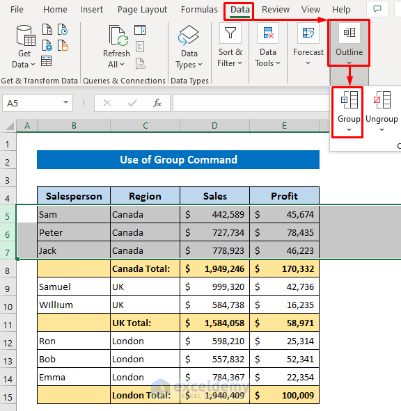
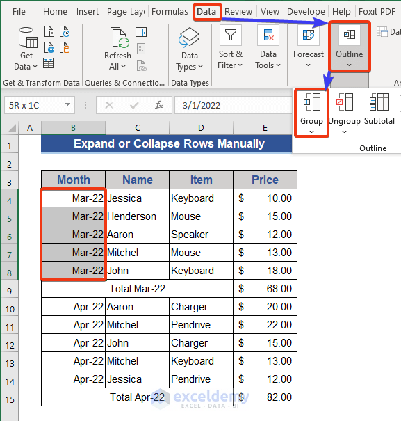
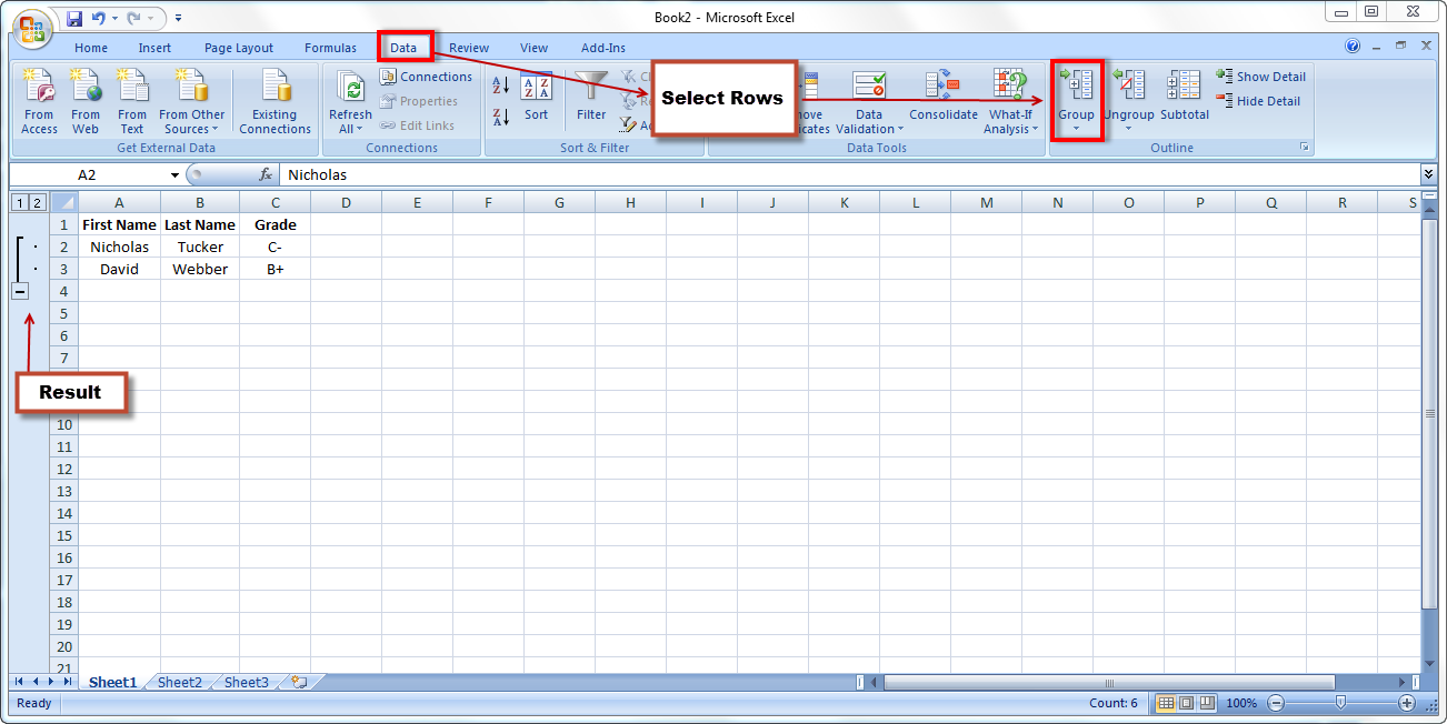
Open your Excel spreadsheet and navigate to the worksheet where you want to apply collapse rows. Select the rows that you want to collapse by clicking and dragging the row numbers on the left-hand side of the spreadsheet. B. Click on the "Group" option under the "Data" tab
How to Group Rows in Excel with Expand or Collapse (5 Methods) (2023)
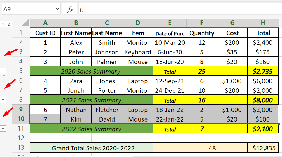
2. Level 1 contains the total sales for all detail rows. 3. Level 2 contains total sales for each month in each region. 4. Level 3 contains detail rows — in this case, rows 17 through 20. 5. To expand or collapse data in your outline, click the and outline symbols, or press ALT+SHIFT+= to expand and ALT+SHIFT+- to collapse. Windows Web
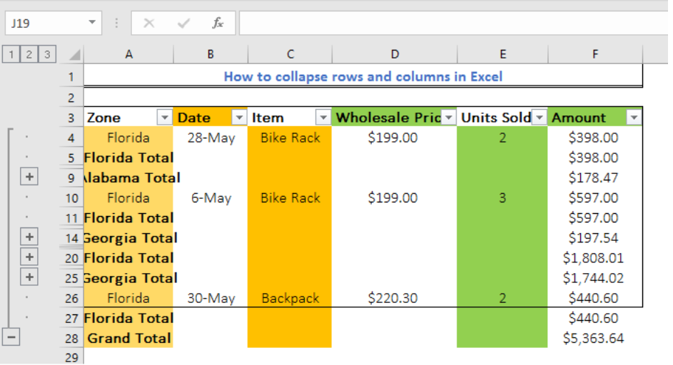
Figure 6 Collapsing rows outline
The quickest way to learn how to collapse rows in Excel is to use the context menu by selecting the rows you want to hide and clicking " Hide ." Read on to learn how to do this by following the screenshots and learning the alternative ways you can collapse and expand rows in Excel. How To Collapse Rows in Excel

How to create collapsible rows in Excel YouTube
Right-click on the selected row (s) and choose "Group" from the drop-down menu. Your rows will now be collapsed, and a small minus sign will appear next to the row numbers to indicate that they are hidden. If you want to unhide the rows, simply click on the plus sign that appears next to the row numbers.
How To Collapse Pivot Table Rows In Excel
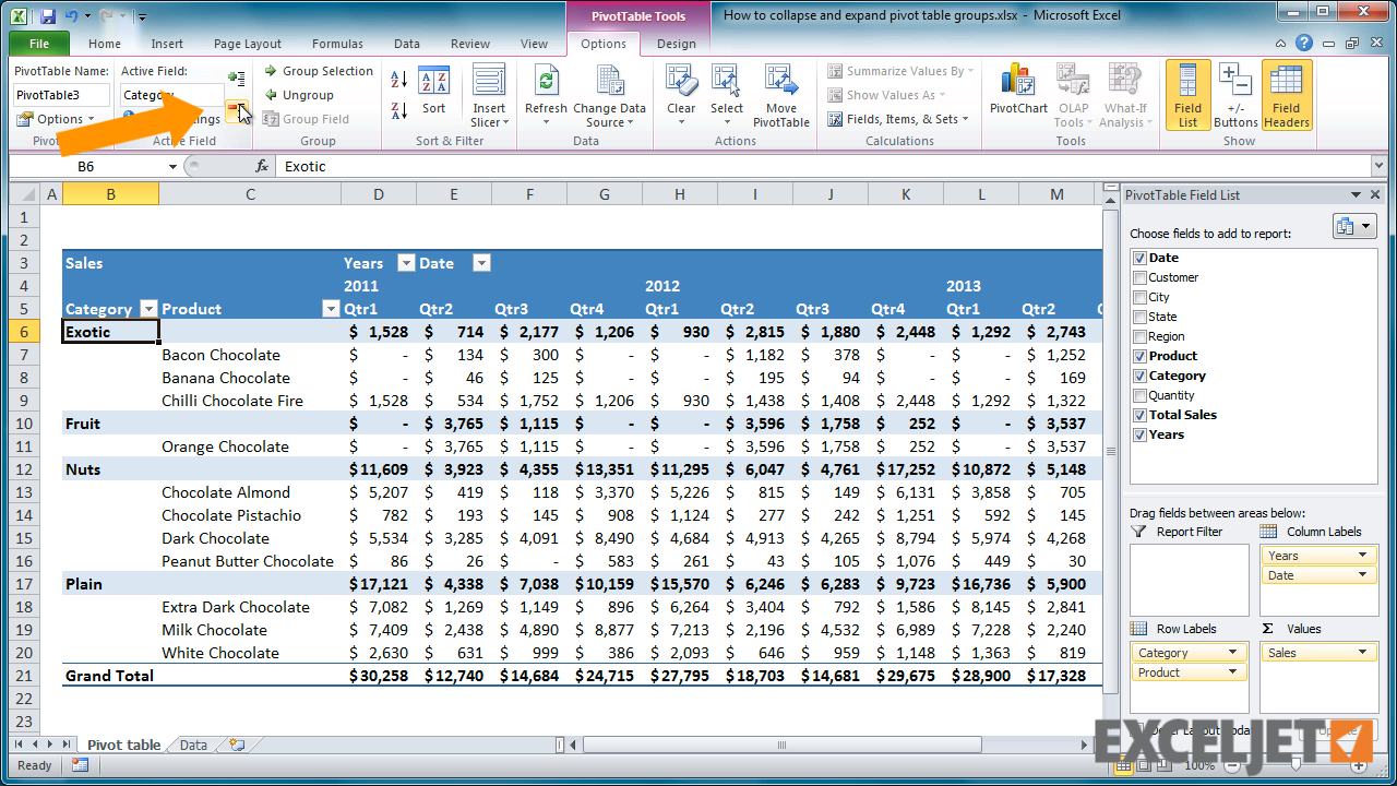
Method 1: Using the Group Feature The first method for collapsing rows is to use the Group feature in Excel. Here's how: Select the rows that you want to collapse. Right-click on the selected rows and choose "Group" from the drop-down menu. You'll see a small icon appear on the left-hand side of the spreadsheet that looks like an arrow.
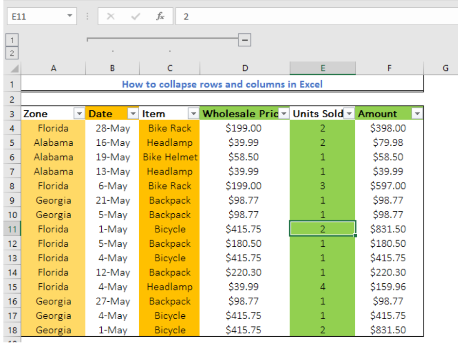
Figure 12 Uncollapse columns
Step 1: Open your Excel spreadsheet and navigate to the worksheet containing the rows you want to collapse. Step 2: Click on the row number on the left-hand side of the spreadsheet to select the entire row. You can select multiple rows by holding down the "Ctrl" key while clicking on the row numbers.
Excel tutorial How to collapse and expand pivot table groups
Method 1: Grouping Rows Select Rows: Open your Excel spreadsheet and identify the rows you want to collapse. Click and drag to select the rows. For example, if you want to collapse rows 5 to 10, select those rows. Group Rows: Right-click on the selected rows. Choose "Group" from the context menu.

2 Methods to Collapse Rows in Excel QuickExcel
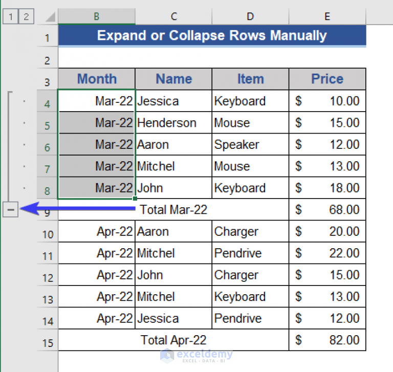
Collapse Rows in Excel To collapse rows in Excel, you have to first group your dataset. Here, we are grouping our dataset manually. To group rows in Excel, we can either use an auto outline or group manually. There is a basic difference there. You must have some subtotal rows to apply auto grouping whereas you can apply manual grouping in any case.

How To Create Collapsible Rows In Excel Latest Tips Picks 2023 Otosection
December 9, 2023 manycoders Key Takeaway: Collapsing rows in Excel is a great way to simplify and organize large spreadsheets. By grouping rows together, you can focus on specific sections and easily navigate the document. There are two main ways to collapse rows in Excel.

How To Collapse Rows In Excel Pixelated Works
How to Collapse a Grouped Row Note the buttons on the left side of your grouped rows. You'll use these buttons to collapse and expand your group. To collapse the group, click the minus (-) sign or button 1. To expand the group again, click the plus (+) sign or button 2. How to Use Subgroups, Additional Groups, and Subtotals

Excel Collapse Rows How to Use Collapse Rows Feature Earn & Excel
To group rows in Excel manually: Select the rows to group together. Navigate to the Data tab. Press the Group button to group the selected rows. Grouping rows allows you to show and hide parts of your data with a single click (we'll show you how to do that later on in this post). This makes it easy to focus on specific sections of a large.
How To Collapse Values In Pivot Table
Select the rows that you wish to collapse, then click on the Data tab and Groups in the Outline group, and then click on Group Rows. You will see a '-' sign on the left of column A. When you click on the '-' sign, the selected rows get collapsed. Now the '-' sign changes to '+' which denotes that the rows are hidden.
How to Expand or Collapse Rows with Plus Sign in Excel (4 Easy Methods)
Select the rows you want to collapse by clicking on the numbers on the far left of the sheet to highlight the entire row. Choose 'Hide' from the quick-menu option. Right-click on your selections and click the 'Hide' button within the context menu.
Excel Spreadsheets Help How to create collapsible rows in Excel
Method 3: Use Auto Outline Command to Group Rows in Excel with Expand or Collapse. In the previous methods, we had to make groups separately for different regions. But using this method we'll be able to group all rows based regions at a time. Select any data from the dataset. Later, click as follows: Data > Outline > Group > Auto Outline.